The goal of this article is to introduce a few commonly used methods of evaluating machine learning classification models, and when one may want to choose a particular performance metric over the others. The hope is that this article could be useful to both beginners looking for an introduction to some of the performance metrics available, as well as intermediate users looking for a refresher or some example applications.

The following metrics are covered in this article (click a link to jump directly to that section):

The Machine Learning Process

Before diving into the wide selection of model evaluation metrics at our disposal, it’s first important to have an idea of where this fits into the overall machine learning process. A typical process may look like this:

The data preparation stage of the modeling process consists of:

Acquiring and cleaning a dataset
Engineering “features” or variables out of the cleaned data
Dividing the whole dataset into a training and testing dataset (or a training, testing, and validation dataset in many cases).

Using the training set, we then try to build an algorithm that learns how combinations of a datapoint’s features relate to that datapoint’s classification. For example, if we’re building a model that predicts if a song will be a number one hit on the Billboard chart, we might find that the song’s genre or artist’s popularity plays a strong role in making this prediction, where the song’s length may be less useful in making this prediction.

Evaluation metrics become especially useful in giving us a single metric indicating how well our model makes predictions. This can be especially useful in two ways:

Optimizing the model during training: choosing the right evaluation metric tells our model what we should be optimizing towards during the training stage
Evaluating the model in the real world: selecting the right metric helps us to see how well we might expect our model to perform in the real world, and ensures that the expected performance aligns with our business goals

The machine learning process is also highly iterative, often requiring many ongoing tweaks and adjustments to get the best performance possible. Evaluation metrics allow us to track and quantify how much any changes we make to the model impact performance.

It’s important that evaluation metrics are selected correctly from the start, as the selected metric should remain consistent throughout the ML process (but don’t be afraid to change the metric if business goals also change). This article should hopefully provide an introduction to some commonly-used evaluation metrics, as well as some guidelines on when you may prefer to use one over others for specific applications.

Accuracy

Very simply, accuracy is the percentage of times that our model makes a correct prediction. To put this into context, we can consider an example.

Suppose we want to build a model to classify our data into one of two possible categories (or classes). We’re given some characteristics of each datapoint (feature #1 and #2), and we use those characteristics to train a model that learns associations between the two features and the class type. In this case, our model attempts to create a linear separation between the two classes, as shown below.

We find that the model we’ve trained is able to identify a pretty useful separation between the two classes, but it’s not perfect due to some overlap between the two groups. The model creates a linear decision boundary, for which any datapoint above the decision boundary is classified as Class 1, where any datapoint below is assigned a Class 2 prediction. With this decision boundary, we can see that of the 100 datapoints considered in the figure above, 80 of them are classified correctly, yielding an accuracy score of 80%!

Limitations of Accuracy Scores

Although easy and often useful to calculate, accuracy may not always be the best metric to use when assessing a model’s overall performance. This is especially true when it comes to imbalanced classes. To show this point, let’s consider a model that’s designed to help a bank detect fraudulent credit card transactions. We take a sample of 100,000 total credit card transactions and out of those, we find that 1,000 of them are fraudulent.

If we pick a model that predicts non-fraudulent on every transaction, then we achieve an accuracy score of 99%, but it fails to ever detect a single case of fraud. In a case like this, an extremely high accuracy score doesn’t tell us the whole story, and we really want to build a model instead that’s effective at detecting those fraudulent cases.

Fortunately, there are plenty of other metrics to choose from - So let’s get into it!

Precision & Recall

Precision and Recall are helpful to use if you want to put more weight on either false positives or false negatives. In the example of a fraud detection model, these types of errors are defined as follows:

A false positive (FP), also known as a Type I Error, is an instance where the model predicted positive when the true value was actually negative. This would occur when a fraud detection model predicted fraud on a non-fraudulent transaction.
A false negative (FN), also known as a Type II Error, occurs when the model predicts negative when the true value is actually positive. This would be the case when a fraud detection model predicted a legitimate transaction when it was actually fraudulent.

Confusion Matrix

A confusion matrix is a great way of measuring performance of a classifier when accuracy alone just doesn’t tell us enough. It allows us to dig deeper to see where things are going wrong if our model’s accuracy score is low, or what we might be missing if our model’s accuracy is high.

To illustrate the concept of a confusion matrix, let’s revisit the same fraud detection example in the previous section. Suppose that we build a model that for the most part predicts transactions to be non-fraudulent, but does correctly identify a fraudulent transaction on occasion. We can use a confusion matrix to get a better read on where our model is making correct or incorrect predictions.

Of the 1,000 total fraudulent transactions of our dataset, our model was able to correctly identify 10 of them (TP). However, not all of the predictions are perfect - there are also 10 non-fraudulent transactions that our model incorrectly identified as fraudulent (FP). For this particular model, we still see an accuracy score of 99%, but by looking at a confusion matrix, we start to get a better sense of where our model is going wrong.

So if a high accuracy isn’t giving us what we’re looking for, what can we consider instead? That’s where precision and recall come into play!

Precision

Precision is defined as the number of True Positives (TP) divided by the number of Predicted Positives (TP + FP). For our fraud prediction example, precision seeks to answer the question:

Out of all the transactions that our model says are fraudulent, what percentage of them are actually fraud?

We want to maximize the precision score of our model when direct costs are high. In other words, if we predict something to be true, we want to make sure that we’re right about that prediction. One excellent use case for maximizing precision is an email spam detector. In this application, we’d much rather let some spam through incorrectly than send important emails to a spam folder. Incorrectly labelling an important email as spam carries the highest risk to the user.

Recall

Recall is defined as the number of True Positives (TP) divided by the number of Actual Positives (TP + FN). For our same fraud prediction example, recall seeks to answer the question:

Out of all the fraudulent transactions that actually occurred, what percentage of these were identified by our model?

Typically, we’d want to train a model that maximizes recall score when opportunity costs are high, or when we want to be sure that our model finds as many actual positive cases as possible, even if it’s wrong sometimes. This is so far the best metric to use in our fraud detection model, but another common example of when we’d want to maximize recall is for cancer detection. Ideally in this case, we’d want to make sure our model detects when someone has cancer every time, even if that means sometimes we raise a false alarm when someone doesn’t actually have it. Being unable to detect an actual case of cancer with our model carries the highest risk.

With what we know now, we can see what our precision and recall scores look like for our “highly accurate” fraud detector model.

Precision = TP / (TP + FP) = 10 / (10 + 10) = 50%

Recall = TP / (TP + FN) = 10 / (10 + 990) = 1%

So we can see that, although we achieve an accuracy score of 99%, we should really be optimizing towards recall for this specific use case. Clearly a lot of work needs to be done still, and it would be useful to shift our strategy to optimize our model to maximize recall.

However, we may not want to only maximize recall. Imagine a scenario where we train a model that predicts every transaction to be fraudulent. While we would be able to catch every fraudulent case, it would cause our users lots of headaches if they’re informed of fraud on their credit card every time they buy something. It might be better to have a more balanced metric that leans towards maximizing recall, but also penalizes the model when precision is very small.

Fortunately, theres a metric for that - the F1-Score!

F1 - Score

The F1-score is great if we want to use some combination of precision and recall in how we evaluate our model. It’s calculated as the harmonic mean of precision and recall. We use a harmonic mean because it allows us to penalize cases where either precision or recall is close to zero. The chart below shows how the harmonic mean behaves differently from a typical, arithmetic mean for different values of precision and a constant recall score of 70%.

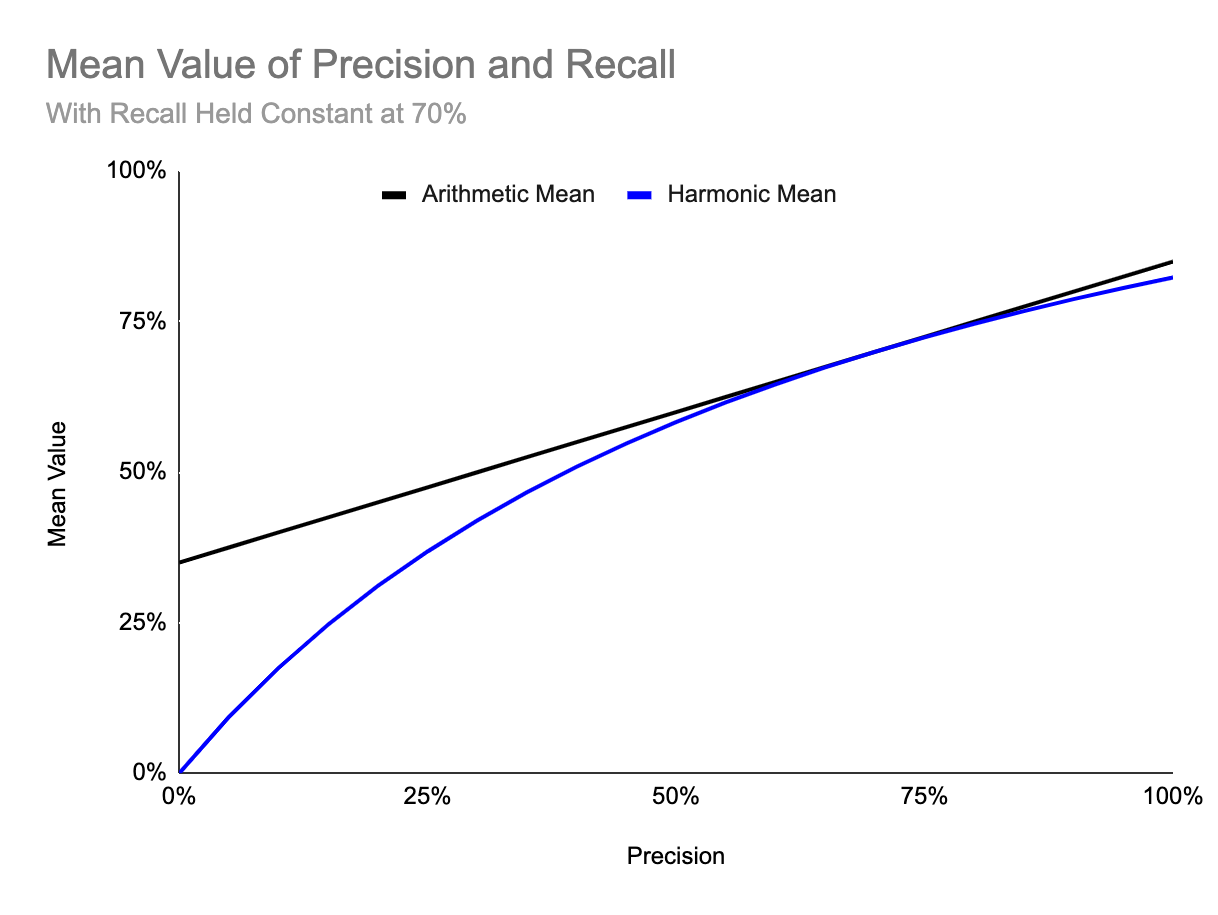
As we can see, when precision is relatively close to the 70% recall score, the harmonic mean (or F1 score) is fairly close to the arithmetic mean of recall and precision. However, notice that when precision is very close to 0%, our F1 score would be 0% as well, despite still having a high recall. The F1 score just makes it easier to observe if either precision or recall is extremely low when we evaluate our model.

Generalized F Score

It can also be helpful to have a more general equation for a weighted combination of precision and recall if one metric should be weighted more highly than the other. This could be useful in our fraud detection model, where we may want to treat recall as our primary metric, but give some weight to precision to reduce our number of False Positives. To apply this weighting, we add a coefficient beta to our equation:

in this case, adjusting our beta value between 0 and infinity allows us to put more weight on either precision or recall. For example, if we set beta less than 1, our F Score will put a higher weight on precision, where setting beta to a value above 1 would weight the F Score in favor of Recall. Setting Beta equal to 1 weights Precision and Recall equally, and just returns the same equation as the F1-Score!

Cost Matrix

While traditional classification models assume that all types of classification errors have the same cost, sometimes it’s useful to consider more specific costs of individual classification errors when evaluating a model. This is especially useful for models that:

Are highly cost-sensitive (as is the case in credit card fraud)
Are trained on data where costs vary on a sample-by-sample basis (for example, a retention model where losing some types of customers carries a higher cost than losing others).

Let’s take a look at this concept in the context of a retention model.

Suppose we’re Data Scientists at a company that runs a subscription-based web service, where customers pay an annual fee to use our product. We’re tasked with building a model trained on demographic and behavioral features to identify customers that are likely to cancel their membership when it comes time to renew. For those we identify as at high risk of cancel, we can offer them a 20% membership discount to persuade them to renew their membership*.

* Note that for simplicity sake, we’ll assume that this promotion will always be enough to convince the customer to renew. However, in the real world, typically more analysis or testing is needed to optimize the actual promotion being offered.

To optimize our model, we could simply look at precision and recall to assess how our model is performing, but in this case we have tangible costs involved, so we could actually assess how cost effective our model is to the business, and even attempt to optimize our model towards this. To calculate cost effectiveness, we need to understand the different costs associated with our promotions:

If we offer a promotion to a customer that was not going to end their membership, then we have a sunk cost of the amount of that promotion. Therefore, anytime we mark a happy customer as at high-risk of canceling their membership (i.e. a false positive), we’ve unnecessarily spent money to retain them.
If we fail to offer a promotion to a customer that was going to cancel (i.e. a false negative), we lose the customer’s business. We can assume the cost here would be losing that customer’s annual membership fee.
On the other hand, if we correctly identify a customer that was going to cancel (i.e. a true positive), we still have to factor in the cost of the promotion, but we gain their business for the next year (along with their annual membership fee)!

We can start to see how costs and rewards can be attributed to each quadrant in the confusion matrix. This allows us to build what’s known as a cost matrix.

To calculate the total cost in each quadrant of our cost matrix, we multiply the calculated cost by the number of cases within each matching quadrant in the confusion matrix. The sum across all quadrants gives us the total cost after implementing the model.

Then, to calculate the cost effectiveness of our model, typically we would compare the total cost savings after implementing our model to the total cost savings when a naive model is used. In this case, a naive model could be whichever of the following carries the lowest expected cost:

A model that always predicts a customer as high-risk, thus offering a promotion to every one of our customers
A model that always predicts a customer as NOT high-risk, thus offering no promotion to any of our customers
A model that uses some sort of rules-based decision method (e.g. only offer a promotion to customers that use the product 3 times per week)
Any historical data we have on retention costs (calculated using an earlier model or alternative method)

$Cost\ Savings = 1-\frac{Costs}{Costs_{Naive Model}}$

If our trained model results in a lower total cost, then we’ll see a positive cost savings - the higher the savings, the more cost effective our model is! Otherwise, our cost savings will be negative, indicating that implementing the model would actually be more costly to the company.

Extensions of the Cost Matrix

The great thing about the cost matrix is that it can also account for cases where cost and reward vary on a sample-by-sample basis. For example, suppose in our example that we offer a set of different, tiered subscription options at different price points (for example, a ‘basic’, ‘standard’, and ‘professional’-tier membership option).

In this case, we can still apply a cost matrix, and the total of each quadrant will automatically factor in these different price points, depending on the types of users that fall into each quadrant. This is one key benefit of this method compared to simply looking at precision, recall, or an F1-Score. Using a cost matrix can allow us to tune a model with cost-oriented goals in mind, and allow us to prioritize sending promotions to one particular set of high value customers over the others in our targeting strategy.

Summary

There are many ways in which a predictive model’s performance can be evaluated, and the method selected should be tailored to the specific application. While I hope this article can provide a useful introduction, this is by no means was this an exhaustive list of everything out there. For now, I’ll provide links for further reading here, but may return to include these in a Part-2 post!

Stay tuned for more, and as always, feel free to get in touch with any thoughts, comments, or questions!